Using/Specifying Reference Data • CanEpiRisk

Installation

library(CanEpiRisk)

1. Overview

This vignette explains how to use the built‑in reference datasets (baseline cancer mortality and incidence rates) and how to provide your own reference data in the format expected by CanEpiRisk.

2. Quick start

(1) Predefined reference data

Regions

Both Mortality and Incidence are lists of length 5 corresponding to WHO-like global regions:

"Aus-NZ Europe Northern America"
"Northern Africa - Western Asia"
"Latin America and Caribbean"
"Asia excl. Western Asia"
"Sub-Saharan Africa"

Show region names:

names(Mortality)
#> [1] "Aus-NZ Europe Northern America" "Northern Africa - Western Asia"
#> [3] "Latin America and Caribbean"    "Asia excl. Western Asia"       
#> [5] "Sub-Saharan Africa"
names(Incidence)
#> [1] "Aus-NZ Europe Northern America" "Northern Africa - Western Asia"
#> [3] "Latin America and Caribbean"    "Asia excl. Western Asia"       
#> [5] "Sub-Saharan Africa"

Sites and object structure

Each regional element is itself a list of site-specific data.frames. The names of the sites available for Mortality data are:

names(Mortality[[1]])
#>  [1] "esophagus"     "stomach"       "colon"         "liver"        
#>  [5] "pancreas"      "lung"          "breast"        "prostate"     
#>  [9] "bladder"       "brainCNS"      "thyroid"       "all_leukaemia"
#> [13] "all_cancer"    "allsolid-NMSC" "allsolid"      "leukaemia"    
#> [17] "allcause"      "survival"

The canonical columns of each site-specific data.frame are:

age (integer, 1–100)
male (numeric)
female (numeric)

Rates are provided on a one‑year age grid (ages 1–100), which are linearly interpolated from corresponding 5‑year rates in the original source (for the highest age category (e.g., 85 or older), the rates are fixed). Some tables (e.g., allcause) may also include person‑years columns (male_py and female_py), which may be used for population-based averaging of calculated risks.

Example (Region 1, all solid cancer mortality):

head(Mortality[[1]]$allsolid)
#>   age         male       female
#> 1   1 3.993729e-06 3.302123e-06
#> 2   2 1.198119e-05 9.906370e-06
#> 3   3 1.996865e-05 1.651062e-05
#> 4   4 1.946148e-05 1.625391e-05
#> 5   5 1.895432e-05 1.599719e-05
#> 6   6 1.844715e-05 1.574048e-05
tail(Mortality[[1]]$allsolid)
#>     age       male     female
#> 95   95 0.02189662 0.01180741
#> 96   96 0.02189662 0.01180741
#> 97   97 0.02189662 0.01180741
#> 98   98 0.02189662 0.01180741
#> 99   99 0.02189662 0.01180741
#> 100 100 0.02189662 0.01180741

Example (Region 3, leukaemia mortality):

head(Mortality[[3]]$leukaemia)
#>   age         male       female
#> 1   1 4.066002e-06 3.390723e-06
#> 2   2 1.219801e-05 1.017217e-05
#> 3   3 2.033001e-05 1.695362e-05
#> 4   4 2.103463e-05 1.704913e-05
#> 5   5 2.173925e-05 1.714464e-05
#> 6   6 2.244387e-05 1.724015e-05
tail(Mortality[[3]]$leukaemia)
#>     age         male       female
#> 95   95 0.0004455293 0.0002765286
#> 96   96 0.0004455293 0.0002765286
#> 97   97 0.0004455293 0.0002765286
#> 98   98 0.0004455293 0.0002765286
#> 99   99 0.0004455293 0.0002765286
#> 100 100 0.0004455293 0.0002765286

Example (Region 5, all-cause mortality with person-years):

head(Mortality[[5]]$allcause)
#>   age        male      female  male_py female_py
#> 1   1 0.056160846 0.048467260 18761.24  18253.13
#> 2   2 0.009220674 0.007515785 18127.85  17684.38
#> 3   3 0.007183781 0.006129537 17634.31  17232.95
#> 4   4 0.005848985 0.005303171 17194.27  16823.33
#> 5   5 0.004864717 0.004698722 16794.60  16448.30
#> 6   6 0.004105606 0.004193329 16422.67  16095.09
tail(Mortality[[5]]$allcause)
#>     age      male    female male_py female_py
#> 95   95 0.3576011 0.2754637  9.8210   23.4550
#> 96   96 0.3680964 0.2902003  6.9710   16.8780
#> 97   97 0.3780983 0.3040167  4.9220   11.9500
#> 98   98 0.3884477 0.3176900  3.4625    8.3635
#> 99   99 0.3989252 0.3305587  2.4190    5.8265
#> 100 100 0.4149599 0.3458980  1.6845    4.0590

Visualizing baselines

Use plot_refdata() to compare site‑specific baselines across regions:

# Lung cancer mortality across regions (legend top-left-ish)
plot_refdata(dat = Mortality, outcome = "lung", leg_pos = c(0.27, 0.95))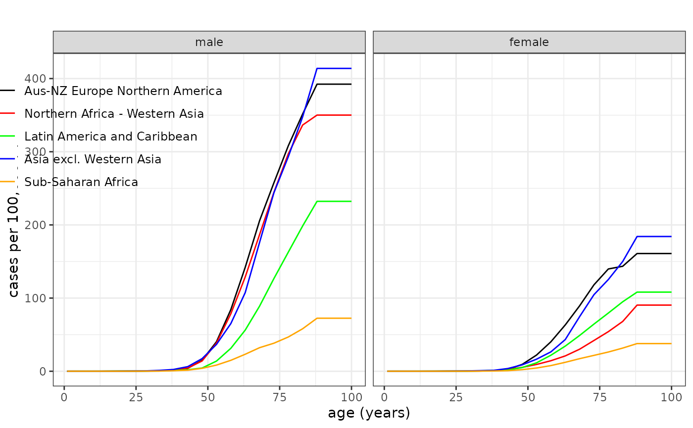

Using reference data in risk calculations

A typical calculation needs a site-specific baseline and all‑cause mortality for the same region:

# Example: CER for all solid cancer mortality (Region 1), female,
# 0.1 Gy at age 15, follow to age 100, ERR model
exp  <- list(agex = 15, doseGy = 0.1, sex = 2)

ref  <- list(
  baseline  = Mortality[[1]]$allsolid,  # site baseline
  mortality = Mortality[[1]]$allcause   # all-cause mortality
)

mod  <- LSS_mortality$allsolid$L       # example risk model (linear ERR)
opt  <- list(maxage = 100, err_wgt = 1, n_mcsamp = 5000)

cer  <- CER(exposure = exp, reference = ref, riskmodel = mod, option = opt)
cer * 10000
#>         mle        mean      median  ci_lo.2.5% ci_up.97.5% 
#>    156.0667    157.7446    156.0157    115.7108    211.9025

Notes: - sex is typically coded 1 = male, 2 = female. - err_wgt = 1 yields pure ERR; 0 would be pure EAR (when available).

(2) Providing your own reference data

You may replace the built‑in region lists with your own. CanEpiRisk expects a list-of-regions, where each region is a named list of sites, and each site is a data.frame with at least age, male, female columns on ages 1:100.

Minimal template

# Build a custom region with two sites as an example
my_region <- list(
  allsolid = data.frame(
    age    = 1:100,
    male   = rep(0, 100),  # replace with your rates
    female = rep(0, 100)
  ),
  allcause = data.frame(
    age       = 1:100,
    male      = rep(0, 100),
    female    = rep(0, 100),
    male_py   = rep(NA_real_, 100),   # optional
    female_py = rep(NA_real_, 100)    # optional
  )
)

Age distribution

CanEpiRisk has an list object agedist_rgn which contains information about the age distribution for each of the WHO global regions. agedist_rgn is used to compute the population-averaged risks using functions population_CER and population_YLL. The age distribution for a WHO global region can be plotted by using function plot_agedist() as below.

# Example: age distributions for Regions 1 and 5
 plot_agedist( regions=c(1,3,5) )
#> Scale for x is already present.
#> Adding another scale for x, which will replace the existing scale.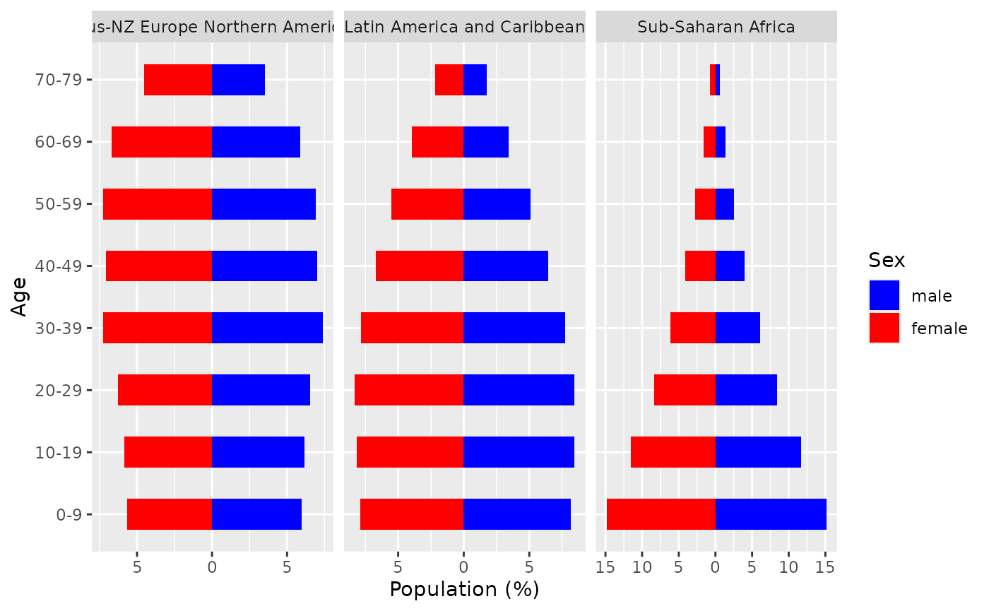

3. Notes

Units: Rates should be per person-year on the age grid. If your sources are in 5‑year groups, aggregate or interpolate to ages 1–100 to match the package convention.

4. See also

Package overview vignette and risk‑model vignette for how baselines are consumed in CER() and related functions.